
| 일 | 월 | 화 | 수 | 목 | 금 | 토 |
|---|---|---|---|---|---|---|
| 1 | 2 | 3 | 4 | 5 | 6 | 7 |
| 8 | 9 | 10 | 11 | 12 | 13 | 14 |
| 15 | 16 | 17 | 18 | 19 | 20 | 21 |
| 22 | 23 | 24 | 25 | 26 | 27 | 28 |
- DP
- 머신러닝
- AI
- 백준
- machine learning
- DynamicProgramming
- 강의정리
- loss
- classifier
- BAEKJOON
- 알고리즘
- 강의자료
- pytorch
- 파이토치
- Hypothesis
- Deep learning
- 파이썬
- Python
- 스택
- Cross entropy
- MSE
- 정렬
- rnn
- Softmax
- 자연어처리
- Natural Language Processing with PyTorch
- 머신러닝 기초
- 딥러닝
- 홍콩과기대김성훈교수
- tensorflow
- Today
- Total
개발자의시작
[Pytorch] 05-2 Logistic Regression 2 본문
글은 모두를위한딥러닝 시즌2 https://github.com/deeplearningzerotoall/PyTorch 을 정리한 글입니다.
GitHub - deeplearningzerotoall/PyTorch: Deep Learning Zero to All - Pytorch
Deep Learning Zero to All - Pytorch. Contribute to deeplearningzerotoall/PyTorch development by creating an account on GitHub.
github.com
Logistic regression은 binary classification 문제
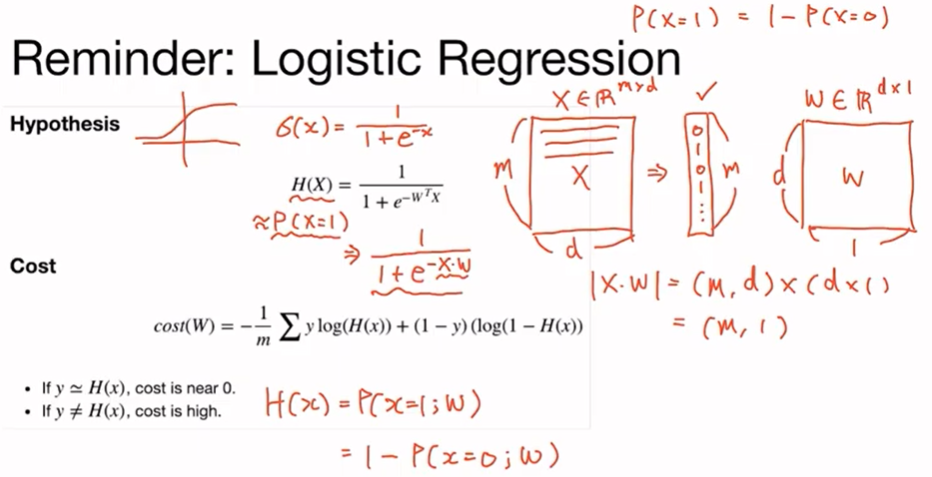
예를 들어 데이터가 X가 주어졌다고 가정할 때 이 데이터는 m개의 샘플로 이루어지고 d의 dimension을 가진 데이터임. 이것을 가지고 m개의 0과 1로 이루어진 정답을 구할 수 있도록 모델을 학습하는 것이 binary classificaion임. 즉 d사이증의 1 dim 벡터가 주어질 때 0 또는 1중 어떤 쪽에 가까운지 구하는 것. 이 경우 정답이 두 개이기 때문에 P(x=1) = 1- P(x=0)로 나타낼 수 있음.
이것을 logistic regression을 통해서 구하게 되는데, 모델의 weight 파라미터(W) 같은 경우는 d x 1 차원이 되고, 데이터 X를 W에 곱해서 0과 1로 나타내야 함. X를 W에 곱한 후 sigmoid 함수를 사용해 0과 1에 근사한 값을 출력함. 결과적으로 m개의 샘플인 데이터 X가 들어왔을 때, H(X)가 0 또는 1이 되도록 하고 싶음. 수식으로 표현하면 |X·W|= (m, d) * (d,1)= (m,1)이 된다. 정리하면 H(x) = P(x=1;w)로 볼 수 있고 이것은 1-P(x=0;w)이다.
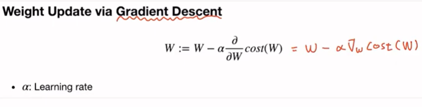
cost는 gradient descent를 통해서 구할 수 있음. weight 파라미터 W에 대해서 미분한 것을 learning rate에 곱하고 이것을 W에서 빼줘서 weight를 업데이트하여 cost를 최소화 할 수 있음.

필요한 라이브러리를 import 한다. 예제에서 똑같은 결과를 재현하기 위해서 torch seed는 고정된 형태로 사용한다.

학습할 데이터는 다음과 같다. x_data의 m=6, d=2 이고 y_data는 m=6, dim=1이 된다.
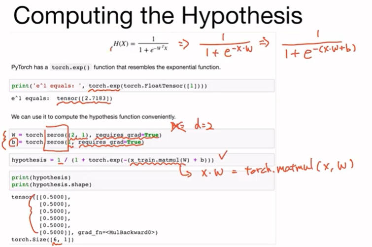
exponential 함수를 torch.exp()함수를 사용하여 구현할 수 있다.

또한, torch.sigmoid() 함수를 사용하여 구현할 수 있다.

cost function은 다음과 같이 정의할 수 있음.

cost funtion을 구현하면 다음과 같다.
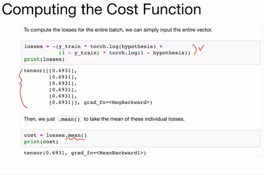
전체 샘플에 대해 구하면 다음과 같이 나타낼 수 있고 6개의 결과를 출력할 수 있음.
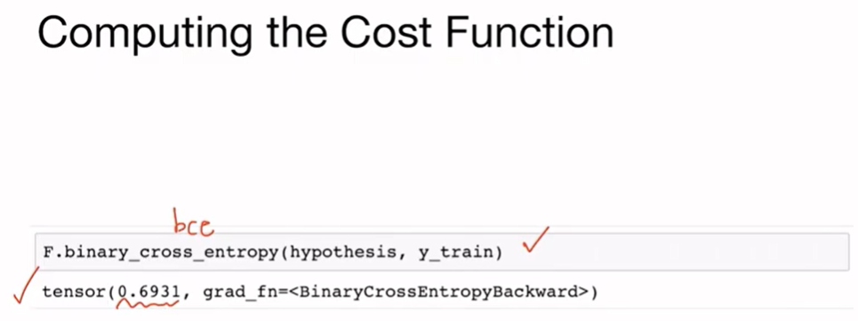
F.binary_cross_entropy() 함수를 사용하여 한줄로 간단하게 나타낼 수 있음.
Code
|
1
2
3
4
5
6
7
8
9
10
11
12
13
14
15
16
17
18
19
20
21
22
23
24
25
26
27
28
29
30
31
32
33
34
35
36
37
38
39
40
|
import torch
import torch.nn as nn
import torch.nn.functional as F
import torch.optim as optim
torch.manual_seed(1)
x_data = [[1, 2], [2,3], [3,1], [4,3], [5,3], [6,2]]
y_data = [[0], [0], [0], [1], [1], [1]]
x_train = torch.FloatTensor(x_data)
y_train = torch.FloatTensor(y_data)
print(x_train.shape)
print(y_train.shape)
print('e^1 equals: ', torch.exp(torch.FloatTensor([1])))
W = torch.zeros((2, 1), requires_grad=True)
b = torch.zeros(1, requires_grad=True)
hypothesis = 1 / (1 + torch.exp(-(x_train.matmul(W) + b)))
print(hypothesis)
print(hypothesis.shape)
print('1/(1+e^1{-1}) equals: ', torch.sigmoid(torch.FloatTensor([1])))
hypothesis = torch.sigmoid(x_train.matmul(W) + b)
print(hypothesis)
print(hypothesis.shape)
losses = -(y_train * torch.log(hypothesis) + (1 - y_train) * torch.log(1 - hypothesis))
print(losses)
cost = losses.mean()
print(cost)
F.binary_cross_entropy(hypothesis, y_train)
|
Whole Training Procedure

Evaluation
(이전과 다른 데이터 사용. github 참고)
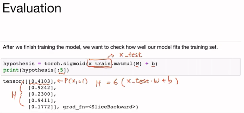
이제 훈련을 했으니 학습된 모델의 성능을 검증한다.

hypothesis가 0.5 보다 크거나 같으면 prediction은 True(1)이 되고 0.5 보다 작으면 False(0)이 된다.

모델의 예측과 실제 정답(y_train)을 비교하면 다음과 같다.

예측과 실제 정답이 일치하는 것을 저장해 주고 이것의 평균을 구하면 모델의 정확도를 알 수 있음.
위의 예제는 BinaryClassifier를 직접 구현해 본 예이고 실제에서 구현할 때는 다음과 같은 형태로 구현하게 된다.

먼저 nn.Module 이라는 추상 클래스를 상속받아 BinaryClassifier라는 logistic regression을 수행하는 모델 클래스를 선언한다. nn.Linear() 형태는 W와 b를 모두 포함하고 있다. 데이터 샘플이 몇 개 들어올지는 상관이 없지만 몇 개의 차원(d)으로 구성되어 있는지는 명시적으로 선언해줘야 한다(8).

|
1
2
3
4
5
6
7
8
9
10
11
12
13
14
15
16
17
18
19
20
21
22
23
24
25
26
27
28
29
30
31
32
33
34
35
36
|
class BinaryClassifier(nn.Module):
def __init__(self):
super().__init__()
self.linear = nn.Linear(8, 1)
self.sigmoid = nn.Sigmoid()
def forward(self, x):
return self.sigmoid(self.linear(x))
model = BinaryClassifier()
# optimizer 설정
optimizer = optim.SGD(model.parameters(), lr=1)
nb_epochs = 100
for epoch in range(nb_epochs + 1):
# H(x) 계산
hypothesis = model(x_train)
# cost 계산
cost = F.binary_cross_entropy(hypothesis, y_train)
# cost로 H(x) 개선
optimizer.zero_grad()
cost.backward()
optimizer.step()
# 20번마다 로그 출력
if epoch % 10 == 0:
prediction = hypothesis >= torch.FloatTensor([0.5])
correct_prediction = prediction.float() == y_train
accuracy = correct_prediction.sum().item() / len(correct_prediction)
print('Epoch {:4d}/{} Cost: {:.6f} Accuracy {:2.2f}%'.format(
epoch, nb_epochs, cost.item(), accuracy * 100,
))
|
'머신러닝(machine learning)' 카테고리의 다른 글
| [Pytorch] 06-2 Softmax Classification Pytorch (0) | 2021.12.29 |
|---|---|
| [Pytorch] 06-1 Softmax Classification (0) | 2021.12.28 |
| [Pytorch] 05-1 Logistic Regression (0) | 2021.12.08 |
| [Pytorch] 04-2 Loading Data (0) | 2021.11.30 |
| [Pytorch] 04-1 Multivariate Linear Regression (0) | 2021.11.30 |


